Photon Behaviour & Cameras

Mr Mars' Camera Resolution Diatribe Page 1 - Photon Behaviour

What is a photon? You can drive yourself mad trying to visualise it. The truth is that nobody really knows.

Photons

There can be no understanding of cameras without some understanding of photons.
The modern idea of what a photon might be was developed by Albert Einstein from 1905-1917. The name "photon" comes from the Greek word for light, and was coined in 1926 by the physical chemist Gilbert N. Lewis¹ as physicists were struggling to get a handle on this slippery fish. A photon is an electromagnetic "wave packet" and can behave as a wave or a particle depending on the experiment. It is fair to say that no one truly understands photons, nevertheless we are able to model their behaviour, and harness them as if we did.

For the purposes of this section a photon is a particle of light. Photons are discrete particles, (ie you can't have half a photon), and are the embodiment of energy in electromagnetic form. Their energy is precisely quantised, (thanks to the quantum theory), and this energy determines the colour of the light. The higher energies are blue, the lower red, and green is in the middle. Light energies extend beyond the visible spectrum but we don't need to cover that here.

Photons of visible light are very small: A green photon has a wavelength of 555 nm. If there were 20 waves in the packet it would be about 1/100 of a millimeter across. Not that you should try and visualise them, they don't follow reality as we know it.
They travel VERY fast: 300,000 km/s, the fastest speed possible for physical objects, (the laws of Physics travel faster).
They contain a VERY small amount of energy. Their energy is proportional to their frequency according to Planck's formula. Green photons have an energy of 3.58×10^-19 J.
There are a LOT of them: This is just as well, since they carry so little energy. A square meter of the earth's upper atmosphere receives around 1300W ^{see footnote 2} of solar radiation when the sun is directly above it, (not all of this reaches the ground). That's 3.6x10²¹ photons per second!

Photon Flux

Now let's tie this back to cameras and establish some benchmarks with respect to photon flux for a range of real world photographic situations involving different pixel pitches and light conditions.

Maximum Photon Flux per Pixel (1/60 sec Exposure)

	Starlight	Tropical Full Moon	Living Room	Storm Dark	European Office	Outdoors Overcast	Bright Day Shade	Full Sun
Illuminance (Lux) ^{see footnote 3}	0.0001	1	50	100	500	1,000	15,000	80,000
Irradiance (Watts/m²)	2.0x10^-7	2.0x10^-3	0.10	0.20	1.0	2.0	30	160
Power per µm² (W)	2.0x10^-19	2.0x10^-15	1.0x10^-13	2.0x10^-13	1.0x10^-12	2.0x10^-12	3.0x10^-11	1.6x10^-10
Energy per µm² per 1/60 sec (J)	3.3x10^-21	3.3x10^-17	1.7x10^-15	3.3x10^-15	1.7x10^-14	3.3x10^-14	5.0x10^-13	2.7x10^-12
Photons per µm² per 1/60 sec	9.3x10^-3	93	4,700	9,300	47,000	93,000	1.4x10⁶	7.4x10⁶

Photons per Pixel - 70 µm² Pixel Pitch	0.65	6,500	330,000	650,000	3.3x10⁶	6.5x10⁶	9.8x10⁷	5.2x10⁸
Photons per Pixel - 35 µm² Pixel Pitch	0.33	3,300	160,000	330,000	1.6x10⁶	3.3x10⁶	4.9x10⁷	2.6x10⁸
Photons per Pixel - 8 µm² Pixel Pitch	0.074	740	37,000	74,000	370,000	740,000	1.1x10⁷	6.0x10⁷
Photons per Pixel - 3 µm² Pixel Pitch	0.028	280	14,000	28,000	140,000	280,000	4.2x10⁶	2.2x10⁷

Enough Photons For Photography?

From this table we can see that yes, full sun means FAR more photons than a night-time living room, and yes, a 70µm² pixel pitch sensor as used by the Canon 5D mk1 gets a lot more photons than the pixels of your typical crap compact of today boasting a 3µm² pitch, (20 times more), that's all as expected. But look at the actual numbers: an SLR shooting RAW stores 14 bits of dynamic range, that's 16,000 different levels. Obviously the levels must go up in at least 1 photon increments, so you might think we just need 16,000 photons per pixel in the bright spots to get a perfectly clean image. (Or we would if the human eye exhibited linear perception. More on this later). Laughing! Even in the living room we have far more than we need. As for the little compact: it only has a 12 bit ADC⁴ so it has a maximum dynamic range of 4,000 levels. Laughing again! It easily makes the bar for the living room case. "FANTASTIC!" you say. All these cameras will take perfect shots right down to your dim suburban living room. ... Won't they?

Sadly, no! Light just doesn't work that way. But remember these benchmark figures, they will be important later. In the meantime make yourself a coffee and strap yourself in, because what comes next is rather complicated.

Poisson Distribution

As a general rule, photons impinging on a surface arrive in a random fashion, much like people ringing a call centre. Although the average number arriving per second is constant, the actual number in any given second varies considerably. This form of behaviour is modelled by the Poisson Distribution, and it is a great bugbear of sensor design and imposes one of the critical limits on image resolution and camera miniaturisation.

Poisson Distribution in a nutshell

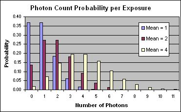
This graph shows the quantum behaviour of light at low intensities. This is a simulation of what a single pixel sees when focused on a white object in low light. The mean photon count is a measure of the intensity of the light, it is the average, (or expected), number of photons striking the pixel in a given exposure.

The "Photon Count Probability" graph uses the Poisson distribution to give the probability of the pixel receiving a number of photons for a given expectation (mean). The blue bars are the probabilities when 1 photon is expected, the burgundy when 2 and the cream when 4. Note how the Poisson distribution approaches a standard distribution as the expected number of hits gets to 4 and beyond.

Poisson Noise

In order to get an accurate image of the subject, each pixel must register the correct colour and intensity. For that to happen each photosite must be struck by the expected number of photons. Now here is the problem: Looking at the graph we can see that when just 1 photon is expected, there is only a 36% chance of getting that outcome, there is an equal chance of getting nothing and an almost equal chance of getting more than 1. If 0 photons corresponds to black, 1 to ¼ tone grey, 2 to ½ tone, 3 to ¾ tone and 4 to white, then your image, which is supposed to be a uniform ¼ grey, will be composed of random dots, 36% black, 36% ¼ tone, 18% ½ tone, 6% ¾ tone and 4% white. A speckly random mess! I have greatly reduced the dynamic range in this example to make the point. In the real world, in your shadows, the speckles won't be at maximum, but they will stand out all the same. Also remember that your pixels are not monochromatic, they are composed of 4 separate photosites (1 each for Red and Blue and 2 for Green), and each one is subject to the Poisson distribution, so you get random colours, as well as random intensities in your noise speckles.

You get the worst speckles when the actual photon count is a long way from the expected. The worst case occurs when you are expecting only 1 photon. As the light intensity rises, the number of expected photons rises, and although there is still variation in how many each photosite receives, the variation is relatively less. By the time you get to an expectation of 4 photons per exposure there is a 90% chance of getting between 1 and 7 photons. This sounds like a bigger variation than the previous example but relatively it is less, because you have widened the pixel definition. If 2-6 photons corresponds to ¼ tone grey and 0-2 photons to black, then 6-10 corresponds to ½ tone, 10-14 to ¾ tone and 14+ white. From the graph you can see that you will now have roughly 17% black, 65% ¼ tone, 17% ½ tone, 1% ¾ tone and almost nothing white. You still have speckles but this is a big improvement.

Image noise at from a real camera at low, low-mid and mid range. D60 ISO1600 4xMag.

Poisson Q Factor

The Poisson Distribution behaves much like a Gaussian (or Normal) Distribution once the mean gets past 20. If we divide the expected number of hits by the width of the main part of the bell, (ie by twice the standard deviation), then we have a measure of the expected relative variation in pixel brightness. This measure is very similar to the electronic engineers' "Q Factor". So close in fact, that I have appropriated the term here even though it is not exactly the same.

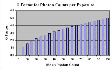
Poisson Q factor for higher counts

This graph shows how the Q Factor increases, as the light intensity increases. A higher Q means less relative variation in pixel brightness and hence a truer image. For example a Q of 2 is reached at an average photon flux of 20. This means that 68% of pixels will receive between 15 and 25 hits, (one standard deviation each side of the mean), 13.6% between 10 and 15, 13.6% between 25 and 30, (taking the next standard deviations), and only 0.3% outside that. We have a 99.7% confidence that when we expect 20 photons, we will get between 10 and 30.

Poisson Aliasing

The issue of large relative variation at low photon counts is quickly resolved by increasing the mean photon flux, but another issue rears it's head when it comes to cameras and that is Poisson Aliasing. Aliasing is where one value is interpreted as another. In this case, where a part of the image that should have a particular intensity is recorded as something else.

It's true that the Poisson Noise (aka Shot Noise) discussed above and the Poisson Aliasing discussed here are really the same thing, but the way they manifest in photographic images and the ways of dealing with them are quite different so I have chosen to differentiate between them. For the purposes of this thesis I shall refer to the extreme chaotic behaviour at very low photon counts as Poisson Noise and the smoother, more insidious behaviour over the rest of the dynamic range as Poisson Aliasing. They are two sides of the one coin that is the Poisson distribution.

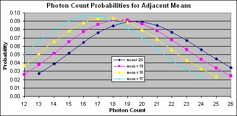
Poisson Aliasing

We can see from this graph how the Poisson probabilities from one mean greatly overlap the adjacent means. To get a correct image, the sensor needs to record the mean level for a given pixel, but the sensor doesn't know what the mean is, it only knows how many photons it received. As we can see from the graph there is no single mean for any given photon count. For example a photon count of 18 could mean a true mean of 16, 17, 18, 19, 20, and others. The probabilities that the true mean is 16, 17, 18, 19, 20 are pretty close, so we really can't expect an image made from simple photon counts per pixel to be accurate.

The only way to get around this problem is to group the photon counts into partitions, where a partition is centered around a given mean with the boundaries set at given confidence limits from the mean. These confidence limits are normally expressed in standard deviations, so that for example, if the boundaries are set at ±1 SD then we have a 68% confidence that if the pixel count lands inside this partition it belongs to the central mean. Later graphs show how this works.

A problem at the bright end

Let us take an idealised camera with 16 bit per colour dynamic range and consider what happens when it takes a picture of an ideal subject that exhibits a matching 16 bit dynamic range. The hot pixels, (those that record the brightest parts of the image) will record 2¹⁶ times more hits than the cold pixels (those that record the black). We need sufficient Q factor so that in most cases, when we are expecting to register the highest value, we don't register the second highest.

If we want each pixel to be 68% right then we must place the pixel boundaries in increments of twice the SD. If we want each pixel to be 99.7% right then they should be in 4x increments. The Poisson Distribution has the unique property that its mean is equal to the square of its standard deviation. This has the effect that to set our maximum pixel count we must multiply the required dynamic range by the partition width in SDs and square the result.

For a 16 bit dynamic range and 4 SDs of width we need 2³⁶ photons hitting the brightest pixel. That's about 6.9x10¹⁰ photons! Well, no camera in the above list is even close to catching that many photons per pixel. If we forget the "almost certain" discrimination level and just shoot for good, we get a figure of 1.7x10¹⁰ photons, still out of the question. This is a good reason not to use 16 bit resolution. The system won't take it.

Today's SLRs only claim 14 bit resolution, but if we allow level partitions 2 SDs apart then we can expect (16,384 x 2)² = 1.1x10⁹ photons at the hot pixels. Again, not even a 35mm sensor in full sun will give you that. Hence we can see that claiming 14 bits of resolution is being unrealistic, but due to modern marketing practices such behaviour has become standard practice for all Manufacturers.

Typically we can expect RAW will provide a maximum of 2 stops each side of an 8 bit per channel JPG. That's 12 bits, so let's see what happens at that resolution.

12 Bit per Channel Intensity Resolution

12 bits of resolution is 4,096 different levels. If we keep the level partitions 2 SDs apart then we can expect (4,096 x 2)² = 6.7x10⁷ photons at the hot pixels. A standard SLR, (APS-C sensor), will catch that many photons per pixel in bright shade or a quality compact in full sun. So we are within sight of the ball park there at least. The standard deviation at the hot end, is 8,192 photons, so our partitions are then twice that or 16,384 photons wide. This means that when we should be receiving 6.7x10⁷ photons, we can have this vary by up to 8,192 photons under or over, and still be classified as the hottest level, that is level 4,096.

I plugged those parameters into a spreadsheet and produced the following graphs to illustrate the point. (Incidentally, for these calculations of the Poisson Distribution with a large mean I had to use the Gaussian Distribution. Not many calculation programs will do 1 million factorial, it's just too big.)

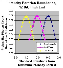
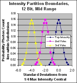
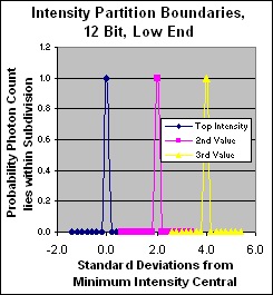
Linear partition discrimination in standard deviations for 12 bit dynamic range

Here we see how well each dynamic level is discriminated from its neighbours. Note that as expected, the problem is at the hot end, although the midrange still exhibits a little cross over. The problematic hot end is separated into quasi-individual bells for each dynamic level although the bells are not fully separated and 32% of received photons still end up in the adjacent levels. However that is a fairly small effect and I doubt it could be seen in the real world. If the max photon count were lowered greatly, we would see much shallower bells overlapping each other in a much stronger fashion at the top end and the loss of discrimination would be visible.

This a reasonable result, but it won't work indoors with an SLR much less with a compact. Nor does it fit the behaviour of the human eye. Time to move on to the next stage of our journey.

If you wish to check my calculations or fiddle with the parameters for yourself then "be my guest"! Here is the spreadsheet.

BTW. You may be saying at this point: "What's all this talk about bright end problems? I know from my camera that most of the noise is in the shadows." Well yes, when you look at finished image that appears to be the case which would appear to contradict this analysis, but I assure you that it does not! The true explanation for this effect is rather complicated and I will deal with it further on when I have covered more ground.

Wikipedia - http://en.wikipedia.org/wiki/Photon.
Wikipedia - http://en.wikipedia.org/wiki/Sunlight
Wikipedia - http://en.wikipedia.org/wiki/Lux
Analog to Digital Converter